Check accessibility while you work in Excel
The Accessibility Checker is a tool that reviews your content and flags accessibility issues it comes across. It explains why each issue might be a potential problem for someone with a disability. The Accessibility Checker also suggests how you can resolve the issues that appear.
In Excel, the Accessibility Checker runs automatically in the background when you're creating a document. If the Accessibility Checker detects accessibility issues, you will get a reminder in the status bar.
To manually launch the Accessibility Checker, select Review > Check Accessibility. The Accessibility pane and the Accessibility ribbon open, and you can now review and fix accessibility issues. The Accessibility ribbon contains all the tools you need to create accessible spreadsheets in one place.
Tip: Use the Accessibility Reminder add-in for Office to notify authors and contributors of accessibility issues in their spreadsheets. With the add-in, you can quickly add reminder comments that spread awareness of accessibility issues and encourage the use of the Accessibility Checker.
Create accessible tables
Tables can help you identify a set of data by name, and you can format the table using styles that make the data stand out. When you carefully name and format your table, you can be sure that everyone can understand your data.
It is also important to specify column header information and use a simple table structure to make sure that screen reader users can navigate the tables easily.
Name a table
By default, Excel names the tables you create as Table1, Table2, Table3, and so on. To make it easier to refer to a table, give each table a descriptive name. A meaningful table name like "EmployeeList" is more helpful than the generic "Table1."
With the descriptive name, you can, for example, quickly jump to the table with the Go To command (Ctrl+G) or the Name Manager dialog box. You can also easily refer to the table in formulas.
-
Place the cursor anywhere in the table.
-
On the Table Design tab, under Table Name, replace the default name, such as 'Table1,' with a more descriptive one.

Note: Table names must start with a letter, an underscore (_), or a backslash (\) and cannot contain spaces.
Select an accessible table style
Light colored tables with low contrast can be hard to read. To make your table more accessible, select a table style that has colors with a strong contrast. For example, choose a style that alternates between white and a dark color, such as black, dark grey, or dark blue.
-
Place the cursor anywhere in the table.
-
On the Table Design tab, in the Table Styles group, select the style you want.
Use table headers
Screen readers use header information to identify rows and columns. Clear table headers provide context and make navigating the table content easier.
-
Place the cursor anywhere in a table.
-
On the Table Design tab, in the Table Style Options group, select the Header Row checkbox.
-
Type the column headings.
Table structures to avoid
Design your tables keeping in mind the following:
-
Avoid blank cells, columns, and rows. When navigating using the keyboard, a blank cell, column, or row might lead a screen reader user to believe there is nothing more in the table.
-
If there is no need for a blank cell, column, or row, consider deleting it.
-
If you cannot avoid a blank cell, column, or row, enter text explaining that it is blank. For example, type N/A or Intentionally Blank.
-
-
Avoid splitting or merging cells: Screen readers keep track of their location in a table by counting table cells. If a table is nested within another table or if a cell is merged or split, the screen reader loses count and can’t provide helpful information about the table after that point. Merged or split cells can make navigating Excel tables with assistive technologies very difficult, if not impossible. Always keep your tables straightforward and simple. To ensure that tables don't contain split cells, merged cells, or nested tables, use the Accessibility Checker.
Use an accessible template
Use one of the accessible Excel templates to make sure that your spreadsheet design, colors, contrast, and fonts are accessible for all audiences. The templates are also designed so that screen readers can more easily read the spreadsheet content.
When selecting a template, look for a template that has several features that support accessibility. For example:
-
Using enough white space makes the spreadsheet easier to read.
-
Colors with contrast make them easier to tell apart for low vision and colorblind readers.
-
Larger fonts are easier for low-vision users.
-
Preset descriptive headings and labels make the spreadsheet easier to understand for users who navigate it with a screen reader.
Add text to cell A1
A screen reader starts reading any worksheet from cell A1. If you have a table on the worksheet, A1 should preferably be the title of the table.
If the sheet is long or complex, add instructions or an overview of the sheet in cell A1. This will inform people who are blind what’s being presented in your worksheet and how to use it. This instructional text can match the background color. This will hide it from people who can see, but allows it to be read by screen readers.
Add alt text to visuals
Alt text helps people who can’t see the screen to understand what’s important in visual content. Visual content includes pictures, SmartArt graphics, shapes, groups, charts, pivot charts, embedded objects, ink, and videos. In alt text, briefly describe the image and mention its intent. Screen readers read the text to describe the image to users who can’t see the image.
Avoid using text in images as the sole method of conveying important information. If you must use an image with text in it, repeat that text in the document. In alt text, briefly describe the image and mention the existence of the text and its intent.
Tip: To write a good alt text, make sure to convey the content and the purpose of the image in a concise and unambiguous manner. The alt text shouldn’t be longer than a short sentence or two—most of the time a few thoughtfully selected words will do. Do not repeat the surrounding textual content as alt text or use phrases referring to images, such as, "a graphic of" or "an image of."
To find missing alt text, use the Accessibility Checker.
Note: For audio and video content, in addition to alt text, include closed captioning for people who are deaf or hard of hearing.
Add accessible hyperlink text and ScreenTips
People who use screen readers sometimes scan a list of links. Links should convey clear and accurate information about the destination. For example, avoid using link texts such as "Click here," "See this page," Go here," or "Learn more." Instead include the full title of the destination page. You can also add ScreenTips that appear when your cursor hovers over text or images that include a hyperlink.
Tip: If the title on the hyperlink's destination page gives an accurate summary of what’s on the page, use it for the hyperlink text.
Use accessible font format and color
An accessible font doesn't exclude or slow down the reading speed of anyone reading a spreadsheet, including people with low vision or reading disability or people who are blind. The right font improves the legibility and readability of the spreadsheet.
Use accessible font format
Here are some ideas to consider:
-
To reduce the reading load, select familiar sans serif fonts such as Arial or Calibri. Avoid using all capital letters and excessive italics or underlines.
-
A person with a vision disability might miss out on the meaning conveyed by particular colors. For example, add an underline to color-coded hyperlink text so that people who are colorblind know that the text is linked even if they can’t see the color.
-
For headings, consider adding bold or using a larger font.
Changing the font size in Excel
Change the default font size for all text
-
Click File > Options.
(In Excel 2007, click
 > Excel Options.)
 -
In the dialog box, click General.
(In Excel 2007, click Popular.)
-
Under When creating new workbooks, in the Font Size box, enter the font size you want.
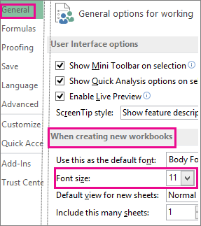
Or, you can type in any size you want, between 1 and 409, in multiples of .5, such as 10.5 or 105.5. You can also choose a different default font style.
Note: To begin using the new default font size or font, you must restart Excel. The new default font and font size are used only in new workbooks created after you restart Excel; any existing workbooks are not affected.
Change the size of selected text
-
-
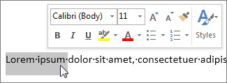
Select the text or cells with text you want to change. To select all text in a Word document, press Ctrl + A.
-
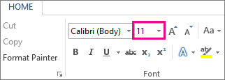
On the Home tab, click the font size in the Font Size box.
You can also type in any size you want, within the following limits:
-
Excel: between 1 and 409, between 1 and 409, in multiples of .5 (such as 10.5 or 105.5)
-
-
Tips:
-
When you select text, a mini toolbar appears near your cursor. You can also change the text size in this toolbar.
-
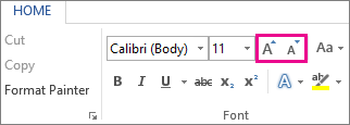
You can also click the Increase Font Size or Decrease Font Size (Grow Font and Shrink Font in some earlier versions of Office programs) icons until the size you want is displayed in the Font Size box.
Use accessible font color
The text in your spreadsheet should be readable in a high contrast mode. For example, use bright colors or high-contrast color schemes on opposite ends of the color spectrum. White and black schemes make it easier for people who are colorblind to distinguish text and shapes.
Here are some ideas to consider:
-
To ensure that text displays well in a high contrast mode, use the Automatic setting for font colors.
-
Use the Accessibility Checker to analyze the spreadsheet and find insufficient color contrast. The tool now checks the documents for text color against page color, table cell backgrounds, highlight, textbox fill color, paragraph shading, shape and SmartArt fills, headers and footers, and links.
-
Use an accessible template.
Create accessible charts
Charts help make complex information easier to understand. To make charts accessible, use clear and descriptive language for the chart elements, such as the chart title, axis titles, and data labels. Also make sure their formatting is accessible.
Format a chart element
-
Select the chart element you want to format, for example, the chart title or data labels.
-
Select the Format tab.
-
Under the Current Selection group, select Format Selection. The Format pane opens to the right.
-
Select the formatting options that make your chart element accessible, such as a larger font or well-contrasting colors.
Rename worksheets
Screen readers read worksheet names, so make sure those labels are clear and descriptive. Using unique names for worksheets makes it easier to navigate the workbook.
By default, Excel names worksheets as Sheet1, Sheet2, Sheet3, and so on, but you can easily rename them.
3 ways to rename a worksheet
-
Double-click the sheet tab, and type the new name.
-
Right-click the sheet tab, click Rename, and type the new name.
-
Use the keyboard shortcut Alt+H > O > R, and type the new name.
Important: Worksheet names cannot:
-
Be blank .
-
Contain more than 31 characters.
-
Contain any of the following characters: / \ ? * : [ ]
For example, 02/17/2016 would not be a valid worksheet name, but 02-17-2016 would work fine.
-
Begin or end with an apostrophe ('), but they can be used in between text or numbers in a name.
-
Be named "History". This is a reserved word Excel uses internally.
Rename a workbook
If you want to rename a workbook, first locate it in Windows Explorer, then you can press F2, or right-click and select Rename, then type the new name.
If your workbook is already open, then you can go to File > Save As to save the workbook with a different name. This will create a copy of the existing workbook.
Delete blank worksheets
Screen readers read worksheet names, so blank worksheets might be confusing. Do not include any blank sheets in your workbooks.
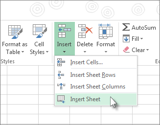
Insert a worksheet
-
Select the
 plus icon at the bottom of the screen.
 -
Or, select Home > Insert > Insert Sheet.
Rename a worksheet
-
Double-click the sheet name on the Sheet tab to quickly rename it.
-
Or, right-click on the Sheet tab, click Rename, and type a new name.
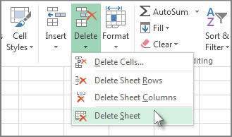
Delete a worksheet
-
Right-click the Sheet tab and select
 Delete.
 -
Or, select the sheet, and then select Home > Delete > Delete Sheet.
Name cells and ranges
Name cells and ranges so that screen reader users can quickly identify the purpose of cells and ranges in Excel worksheets. Users can use the Go To command (Ctrl+G) to open up a dialog box which lists all the defined names. By selecting a name, a user can quickly jump to the named location.
-
Select the cell or range of cells that you want to name.
-
Select Formulas > Define name.
-
Enter the name and select OK.
Note: The name must start with a letter, an underscore (_), or a backslash (\) and cannot contain spaces.
Test the accessibility of your worksheets
When your spreadsheet is ready and you've run the Accessibility Checker to make sure it is inclusive, you can try navigating the spreadsheet using a screen reader, for example, Narrator. Narrator comes with Windows, so there's no need to install anything. This is one additional way to spot issues in the navigation, for example.
-
Start the screen reader. For example, to start Narrator, press Ctrl+Windows logo key+Enter.
-
Press F6 until the focus, the blue rectangle, is on the worksheet table grid.
-
Do the following to test your worksheets:
-
Use the arrow keys to move between the cells in the table grid.
-
To check the worksheet names in your spreadsheet, press F6 until the focus is on the name of the current worksheet, and then use the Left and Right arrow keys to hear the other worksheet names.
-
If your worksheet contains floating shapes such images, press Ctrl+Alt+5. Then, to cycle through the floating shapes, press the Tab key. To return to the normal navigation, press Esc.
-
-
Fix any accessibility issues you spotted when navigating with a screen reader.
-
Exit the screen reader. For example, to exit Narrator, press Ctrl+Windows logo key+Enter.
Note: Also make sure that your worksheets can be easily read on a mobile phone. This not only benefits people who have low vision and use magnification, but it also benefits a very broad set of mobile phone users.
Using a screen reader to explore and navigate Excel
Use Excel with your keyboard and a screen reader to explore and navigate the app main views and elements, and to move between views and functions.
Cycle through the main areas
To navigate between the main areas in Excel, press F6 (forward) and Shift+F6 (backward). The main areas are:
-
Worksheet table grid
-
Sheet tabs
-
Status bar
-
Ribbon tabs
Navigate the ribbon tabs
The ribbon tabs are the main menu bar of Excel. To reach the ribbon tabs, press the Alt key. With Narrator and NVDA, you hear "Ribbon tabs," followed by the current tab's name. With JAWS, you hear "Upper ribbon." To move between the tabs, use the Left and Right arrow keys. When you reach a tab, a tab-specific ribbon appears below it.
Here's a list of the most common tabs and some examples of what you can do on each tab:
-
Home
Format and align text and numbers, and add new rows and columns.
-
Insert
Insert tables, pictures, shapes, and charts into your worksheet.
-
Page Layout
Set the margins, orientation, and size of the worksheet page.
-
Formulas
Add various functions and formulas to your worksheet.
-
Data
Import data from various sources, sort and filter it, and use data tools such as removing duplicate rows.
-
Review
Check the spelling and accessibility of your worksheet, and collaborate with others using comments and notes.
-
View
Select a view such as Normal View or Page Layout view, and set the page zoom level.
-
Help
Open the Microsoft Excel Help, contact support, and leave feedback.
In addition to the ribbon tabs, you need to access the File menu for some important commands. To open it, press Alt+F. The File menu opens in a new pane. To navigate the main commands, use the Up and Down arrow keys, then use the Tab key and Up and Down arrow keys to navigate the options for that command.
In the File menu, you can start a new workbook, open an existing workbook, save, share, or print the file you're currently working with, and access Excel options. To close the File menu and return to your worksheet, press Esc.
Navigate the ribbon
After navigating to the right ribbon tab as described in Navigate the ribbon tabs, press the Tab key to move to the ribbon and browse its commands and options. You can press Shift+Tab to move backwards. Press Enter to make a selection or press Esc to leave the ribbon and return to your worksheet.
Tip: It is often faster to use keyboard shortcuts to access the commands and options on each ribbon.
Navigate the worksheet
When you open an Excel workbook, the focus is on the worksheet table grid. If you have moved the focus out of the worksheet, press F6 until your screen reader announces a table grid cell location. Here's how you navigate inside the worksheet and between other sheets and workbooks:
-
To move between cells in the table grid, use the arrow keys. Your screen reader announces the column and row of each cell as well as its contents.
-
To open the context menu for the current cell, press Shift+F10. Use the Up and Down arrow keys to navigate the menu, and press Enter to make a selection or press Esc to return to the worksheet.
-
To move to the next or previous worksheet in your workbook, press F6 until you hear the name of the current sheet tab, use the Left and Right arrow keys to find the right sheet, and press Enter to select it.
-
To switch to the next workbook when more than one workbook is open, press Ctrl+F6. Your screen reader announces the name of the workbook.
Tip: To quickly move the focus to the first floating shape such as a text box or an image, press Ctrl+Alt+5. Then, to cycle through the floating shapes, press the Tab key. To return to the normal navigation, press Esc.
Use Search
To find an option or perform an action quickly, use the Search text field.
Note: Depending on the version of Office you are using, the Search text field at the top of the app window might be called Tell Me instead. Both offer a largely similar experience, but some options and search results can vary.
-
Select the item or place in your document, presentation, or spreadsheet where you want to perform an action. For example, in an Excel spreadsheet, select a range of cells.
-
To go to the Search text field, press Alt+Q.
-
Type the search words for the action that you want to perform. For example, if you want to add a bulleted list, type bullets.
-
Press the Down arrow key to browse through the search results.
-
Once you've found the result that you want, press Enter to select it and to perform the action.